|

  
|
||
|
|
||
Shortcut:
| Click |
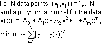
Uses least-squares curve fitting procedures to find the polynomial of a user-specified order that best fits the data. A least-squares curve fit is one in which the sum of the square of the errors between the actual data and the polynomial model are minimized:
DPlot converts the input curve to a form most likely to achieve a good fit (or at least most likely to avoid scaling errors), depending on the type of scaling currently in effect. The actual form of the output polynomial is dependent on the scaling of the plot:
Linear X, Linear Y:
y = C0 + C1x + C2x2 + ... + Cmxm
Linear X, Logarithmic Y:
log10y = C0 + C1x + C2x2 + ... + Cmxm
or
y = 10^(C0 + C1x + C2x2 + ... + Cmxm)
Linear X, Probability Y:
NORMINV(y,0,1) = C0 + C1x + C2x2 + ... + Cmxm
or
y = NORMDISTCDF((C0 + C1x + C2x2 + ... + Cmxm),0,1)
Logarithmic X, Linear Y:
y = C0 + C1log10x + C2(log10x)2 + ... + Cm(log10x)m
Logarithmic X, Logarithmic Y:
log10y = C0 + C1log10x + C2(log10x)2 + ... + Cm(log10x)m
Logarithmic X, Probability Y:
NORMINV(y,0,1) = C0 + C1log10x + C2(log10x)2 + ... + Cm(log10x)m
Probability X, Linear Y:
y = C0 + C1NORMINV(x,0,1) + C2(NORMINV(x,0,1))2 + ... + Cm(NORMINV(x,0,1))m
Probability X, Logarithmic Y:
log10y = C0 + C1NORMINV(x,0,1) + C2(NORMINV(x,0,1))2 + ... + Cm(NORMINV(x,0,1))m
Probability X, Probability Y:
NORMINV(y,0,1) = C0 + C1NORMINV(x,0,1) + C2(NORMINV(x,0,1))2 + ... + Cm(NORMINV(x,0,1))m
where log10 is the base 10 logarithm and NORMINV is the inverse of the cumulative distribution function.
Scale types not specifically mentioned above will use the default linear X, linear Y form.
Note that these conversions performed by DPlot will yield, for example, a straight line for a 1st order fit on any of the scale types mentioned above, though the relationship between X and Y may not be linear. If you want the standard polynomial y = C0 + C1x + C2x2 + ... + Cmxm for a non-linear scale then you should switch to a linear X, linear Y scale before performing the curve fit, then back to the appropriate scale afterwards.
Please note: Points with Y values outside the limits set with Amplitude Limits are ignored. If you want those points to be considered, first turn Amplitude Limits off.
Correlation coefficient
The correlation coefficient presented by DPlot is a measure of how well the polynomial is correlated to the data. A correlation coefficient of 1.0 denotes a perfect fit, while a correlation coefficient less than 0.9 should probably be discarded. A high correlation coefficient less than 1.0 does not necessarily indicate an especially good curve fit (see below).
The correlation coefficient is described mathematically as:
Standard error about the line
The standard error about the line is another measure of the goodness of the fit, and is analogous to standard deviation. A standard error of 0.0 indicates that the curve fit passes through the input data points exactly.
where m = the number of unknowns in the fit (1 for the mean, 2 for a straight line, 3 for a quadratic, etc.)
Limitations
In general, least squares curve fits are very poor predictors of trends in the data outside the limits of the input. Extrapolation outside the limits of the input is not recommended for any but 1st order fits. The figure shown below illustrates the problem associated with extrapolating outside the limits of the input data. Even though the generated curve fits the input perfectly, values outside the limits of the data are, at best, suspect.

Bear in mind that the least squares procedure operates only on existing data points. A generated curve fit might fit the data points exactly, but produce completely unexpected results between data points. This is particularly true for high order polynomials. As in the figure above, the generated curve in the figure below fits the input data precisely. However, in this case, a 1st or 2nd order fit would produce a much more realistic model of the input data, even though the resulting polynomial would not be perfectly correlated.

A high (but less than 1.0) correlation coefficient is not necessarily an indication that a curve fit is appropriate for the input data. Consider the following examples, commonly referred to as Anscombe's Quartet:
|
|
|
|
The input data in each example has a mean Y value of 7.5, a mean X value of 9, a standard deviation in the Y values of 2.03, and a best fit line of Y=3+0.5*X with a correlation coefficient of approximately 0.81. It should be obvious from the above that the correlation coefficient alone is not a good predictor of the goodness of the fit or, especially, the goodness of the fit for one data set relative to another. You should always view a graphical representation of a curve fit before making any judgments concerning the appropriateness of that fit.
|
Related macro commands |
____________________________
See also:
Page url:
https://www.dplot.com/help/index.htm?helpid_curvefit.htm


